Ingesting 10 billion rows of timeseries data in 95 seconds

Timeseries data = ingestion challenges

If there’s one thing that’s hard when managing timeseries data is just the sheer amount of it. Timeseries data has volume built-in because it’s cumulative. You don’t want a single picture: you want the whole movie!

In finance, several terabytes a day is nothing out of the ordinary. Most industrial IoT use cases are just distributed DoS in disguise.

Gartner tells us that half of the data in the world will reside outside of datacenters by 2022. Edge processing will mitigate the amount of data we need to take in, but it’s still A LOT OF DATA.

How to manage that?

In a previous blog post, we wrote about distributed file systems being a decent option when your data IS JUST TOO MUCH. The problem with distributed file systems: well, they don’t have any awareness of the data you’re storing. Which is why we have databases! But databases can’t take all that data in! Ok let’s use a filesystem! But I can’t query my filesystem!

So what do to do?

A timeseries database is supposed to be good at ingesting data, better than a generic relation database that is. And most of them are!

But well, we don’t care about other timeseries databases. Let’s talk about our timeseries database, central to our timeseries offering: QuasarDB!

In this blog post, we’re going to show you how much hardware it takes to ingest more than 100 M rows per second with QuasarDB. We’ll run that in AWS, show you all the options, scripts, and parameters so you can see for yourself that this is, as we say in French, réalisé sans trucage.

The test

We could have written a data generator that writes directly into QuasarDB, but if we knew that if we did that someone would say “Ha! These C++ nerds just did some dark template voodoo in the data importer, it’s not realistic!”.

There’s a timeseries benchmark floating around that has some merit. However, when it comes to ingestion it’s one (if not two) order of magnitude slower than needed to seriously stress our engine.

What’s important with this test is that ingestion must be remote. There are a lot of benchmarks where you just ingest data locally, and they are not measuring interesting things because in real life, at some point, the data was not physically on the same machine as the database.

What we did, is generate CSVs files, and used our off-the-shelf importer tool (qdb_import) codenamed “Railgun” to import that data into QuasarDB. If you’re curious, our export tool (qdb_export) is named “Nugliar,” which is probably a sign that the team should cut back a little on the coffee and sugary drinks.

Using CSV files for this ingestion also has the built-in, “fair” logic of “the data was in a file, on a remote machine, external to the database, and now it’s inside the database”. It’s a realistic data engineering use case.

The CSV file consists of a timestamp, a double, and an integer. Values come out of a pseudo-random number generator based on a linear congruential generator. See what I did there? I could have said it comes from numpy random generator, but I would have looked half as smart, so I didn’t.

In short: we have multiple clients importing the data connecting to a remote cluster handling the data.

The AWS setup

AWS is the environment that we’re the most familiar with (as it’s the infrastructure for our managed solution), and we wanted to have something you, the reader, could reproduce if you wanted to.

Just keep in mind that a 20% performance variation is typical in cloud instances. If that helps, all tests were run in the eu-west-1b AWS datacenter.

The QuasarDB cluster was made of five (5) c5d.18xlarge instances and the remote clients were running on two (2) r5a.24xlarge instances. We put all instances in a single placement group to reduce cloud noise.

All instances were running Amazon Linux 2 HVM (ami-01f14919ba412de34).

QuasarDB indexes and compresses the data as it arrives, so a bit of CPU power is welcomed. To ensure that the clients could send the data fast enough, we loaded the CSVs into memory. An alternative would have been to run more instances in parallel. You’ll see soon enough that the challenge was more about sending the data fast enough than QuasarDB handling it.

Measuring resource usage

To measure the resource usage, we used the built in AWS monitoring system and Datadog, which is what we use for our managed instances as well. If for some reason there is a big difference between what our tools report and what external monitoring sees, we know something is wrong in our test.

The QuasarDB cluster configuration

To install QuasarDB just follow the RPM installation instructions available here.

The QuasarDB setup has nothing special going for it. However, for the sake of making the test reproducible we share the config of the first node.

For the clustering to be configured, each node just needs to reference at least one other node in the cluster in the “bootstrapping_peers” field. For this test we disabled security. Security has no impact on ingress speed, unless you enable full stream encryption (that uses AES 256 GCM).

The most important parameter here is the partition count that we set at 16 for this specific hardware configuration. That means that each node will be able to process at most 16 requests in parallel.

QuasarDB has built in map-reduce, so when you run a query, it’s often fragmented in smaller queries. This smaller query ends up running in one of those partitions. That’s why this partition count parameter is so important; if it’s too low you will underuse the resources available on the machine, if it’s too high you end up overloading the OS scheduler. Learn more in our technical white paper.

The QuasarDB version we used for this benchmark is 3.5 RC2. If you use the above configuration on a 3.4 setup, it won’t work as we introduced some changes in the configuration files.

Last, for each node, you need to have a different node ID, the first one being “1/5”, the second one “2/5”, etc.

The data

The data is generated by the following script.

You end up with 10 billion rows for a total size of 500 GB, the data is split in half on two nodes running Railgun (our importer tool) each.

Note that this random data is unfavorable for QuasarDB, as our compression algorithms perform poorly on random data. The insertion speed we got in this test is thus a lower bound.

The QuasarDB import node configurations

The machines are heavy on RAM because when we did the initial run we realized we were bound by how fast Railgun could read the CSV from disk. To solve that problem, we put the CSV in a RAM FS, that way a single railgun using 96 threads could send the data fast enough.

Railgun has built-in support for multithreading, which prevented running multiple railgun on a single machine to simulate multiple clients. We used the synchronous import mode (the default) as in this context the asynchronous mode wouldn’t bring any benefit.

To be clear about railgun, it has an optimized CSV parser and does a lot of smart stuff to minimize overhead; however the high performance data insertion is done by our batch API that you can use in any program written in a supported language (or that supports C binding).

The shard size chosen for this test is 100ms given that we have one point every microsecond.

The results

Well, we kind of gave it away in the title. To ingest the 500 GB of remote CSV data it took only 95 seconds from start to finish. Most ingress benchmarks measure the database ingestion part only.

Reading, slicing, sending, indexing, compressing, and storing 500 GB of remote CSV data took 95 seconds on this setup.

That’s more than 5 GB per second, on average, or in terms of rows per second more than 100 million of rows per second. To be fair, the actual data being transmitted on the network is much lower as 5 GB per second, because the protocol between the client and the server is using a highly efficient binary representation of the data.

To make it absolutely transparently clear: the data is actually written to disk and visible immediately after acknowledgement. Not only do you ingest as fast as a network file copy would occur, but you can query, aggregate, transform the data, in ways a typical RDBMS can’t (ASOF joins for example).

The final disk usage after the transfer was 80 GB, most of it is due to efficient data representation as most of the data being random, compression can’t be as good as it could.

Resource usage

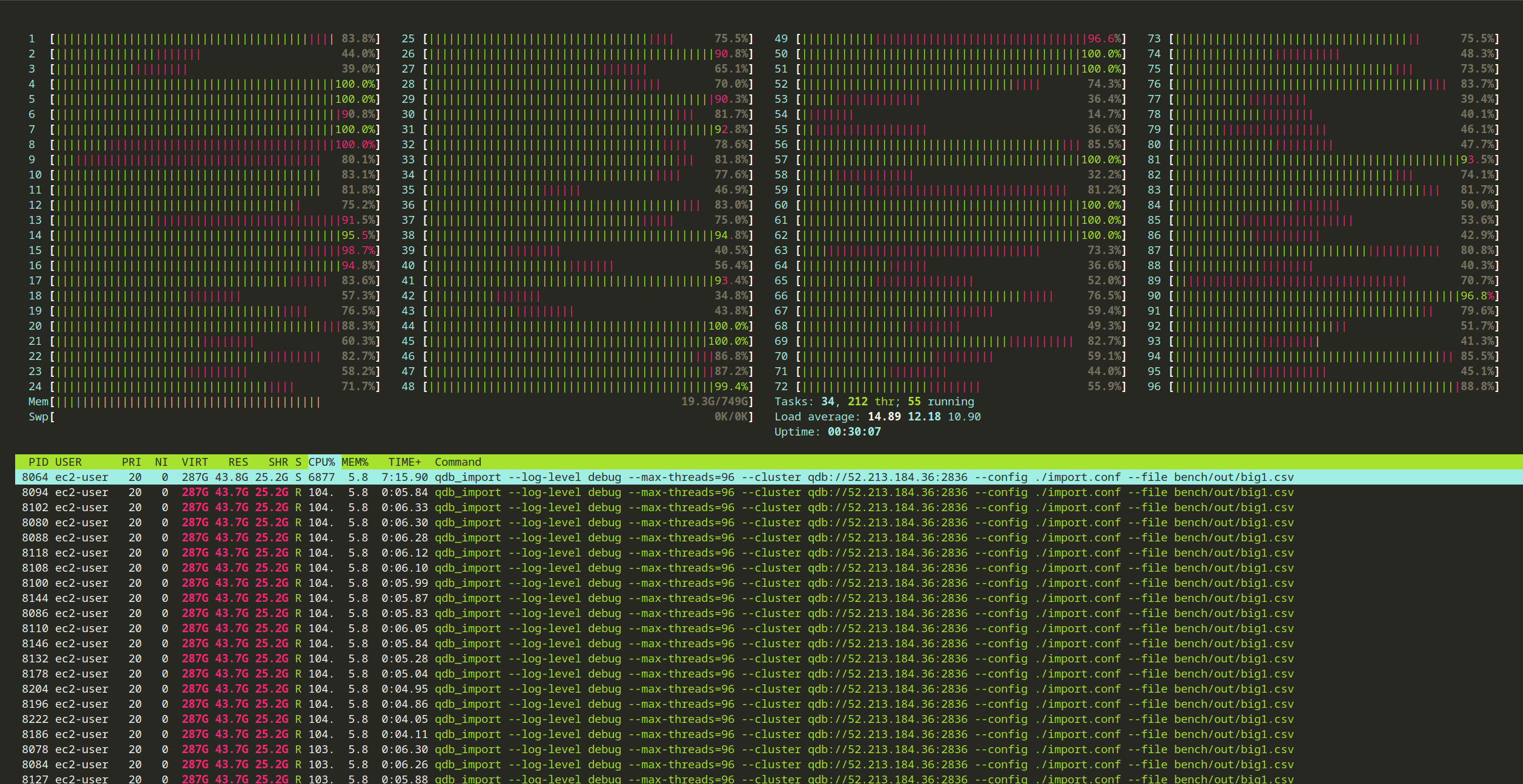
What is more interesting to look at how busy the node. If you look at one of the importers nodes (the nodes that send the data to the cluster), the CPU is usage is very high:

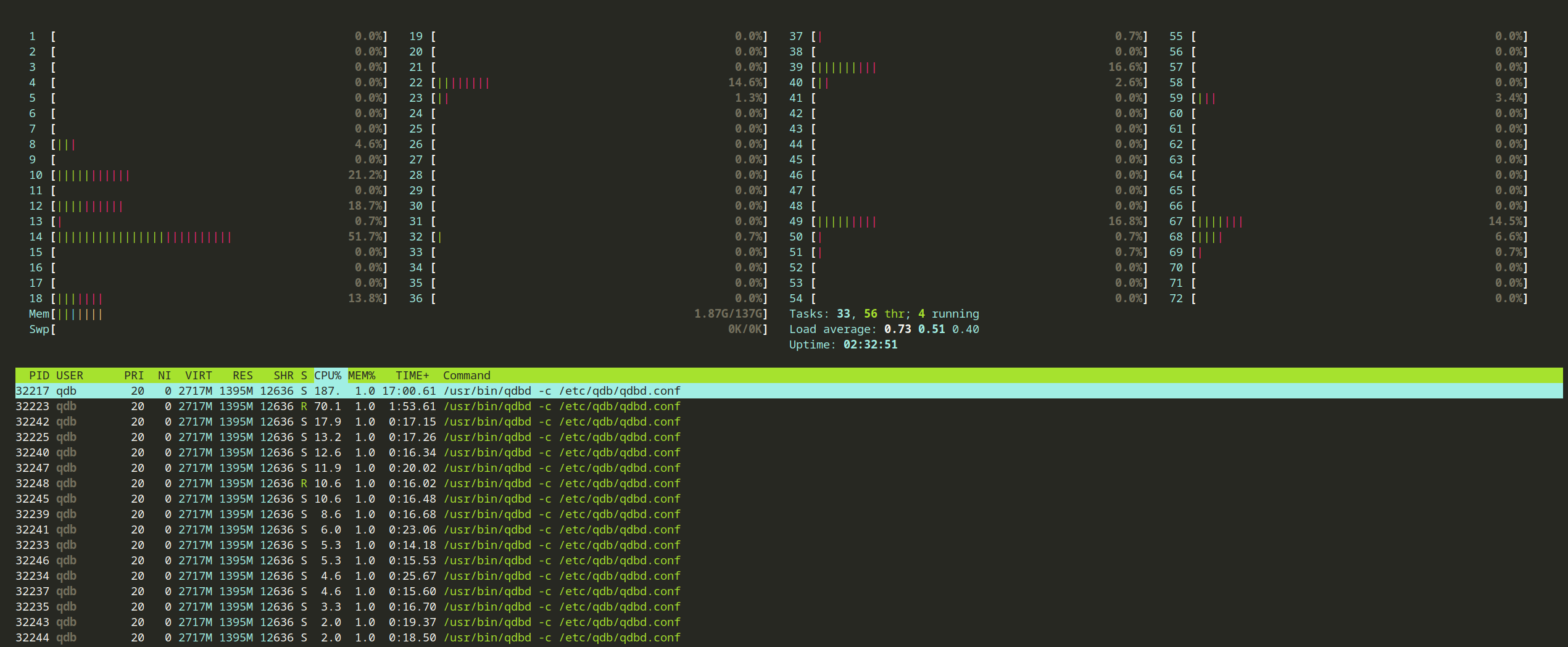
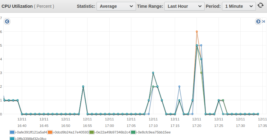
Whereas if you look at a node on the cluster, the usage is very low:

That’s confirmed by the AWS cloudwatch aggregated metrics for the importer nodes:

 

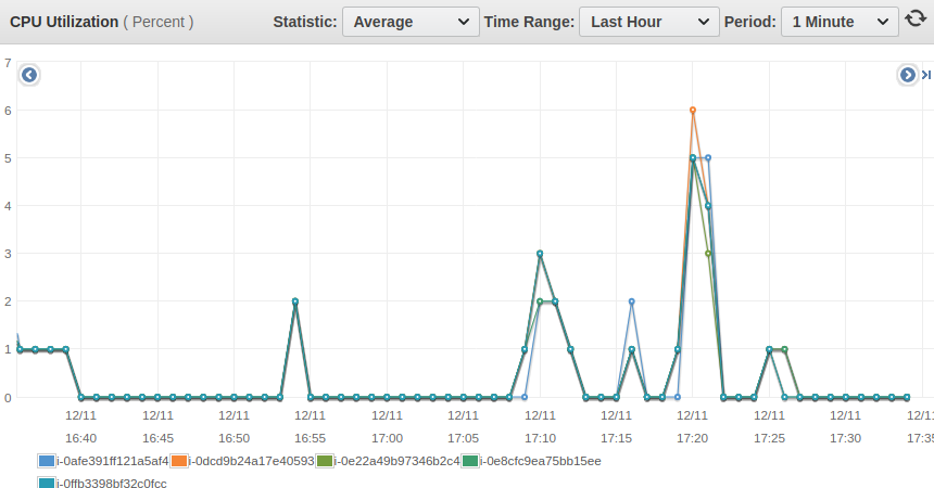
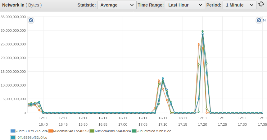
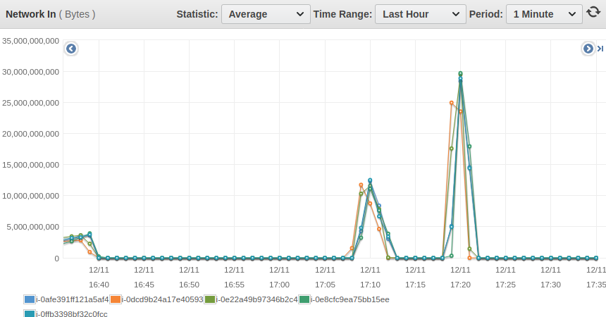
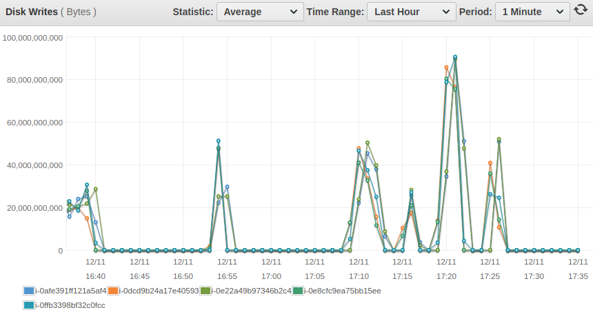
And on the cluster nodes:

 

 

How do we achieve this?

QuasarDB high ingestion speed comes from different things:

• The QuasarDB ingestion API prepares the data in a way that makes verification and insertion of the data by the cluster much faster. That’s the kind of thing a purpose-built timeseries database management system can do. This is great for high ingestion like in this instance, but also extremely important for IoT and edge uses cases as it distributes some of the workload to each node.
• The complexity to lookup the right bucket on a QuasarDB cluster is O(1). The clustering has thus a negligible amount of overhead.
• On the server side, almost every operation is zero copy from network to disk persistence. Our custom indexing and compression algorithm work faster than even the fastest persistence medium there is (as of 2019). If you’re curious about our compression technology, read this article.

Another thing which is hard to list has an objective reason is that just every possible tiny bit of QuasarDB is heavily optimized, with a native C++ implementation leveraging CPU cache structure, memory layout, SIMD instructions whenever possible. On a micro-level, some of these optimizations may look negligible, but all put together they add to the bottom line.

The conclusion

With an average CPU usage of 10%, it seems our five (5) nodes cluster still has a lot of headroom, which makes it tempting to see how far it could go. In a future test, we’ll see what it takes to blast away the billion rows per second barrier.

We’re aware that this test has shortcomings. For example, it isn’t a good approximation of streaming data ingest where data comes in an irregular way. If you’re part of the STAC community, you know we’re working with the rest of the working group on an updated STAC M3 benchmarks that reflect streaming workload better.

If you’d like to test QuasarDB ingestion capabilities for yourself, you can reproduce this test, use our Kafka connector, or write your own program using our batch insertion API.

The community edition does support clustering!

Enjoy the holidays season, and see you in 2020 for even crazier results!