Introducing Delta4C: a high speed, adaptive, lossless compressor for timeseries

This post is part of a series about the challenges behind database performance and how to accurately assess it.

Why compression matters so much for timeseries data

Whatever database engine you are using, efficient disk storage is always welcomed. When your 10 GiB become 100 GiB once in the database, that’s never a nice thing!

What sets apart timeseries from “regular” data is its intrinsic cumulative nature: new data keeps coming in, and you probably want to keep as much history as you can. Thus, timeseries use cases tend to have much larger storage requirements.

The other difference is that timeseries data has obvious patterns and new values often have a high correlation with previous values.

After all, if you recorded one second ago a temperature of 20 °C, the temperature is likely still 20°C.

Understanding compression

Data compression is one of the most heavily studied field in computer science. One can see compression as a trade-off between computing time and storage space.

The best way to understand compression is to go from an example. Let’s have a look at this Python program:

import random
import string

random.seed(0)

with open("random.txt", 'w') as f:

    for i in range(0, 10240):

        f.write(random.choice(string.ascii_letters))

Because we seed the random generator with a constant value, the output is always identical between runs.

If you compress the file with zip or a similar utility, you will obtain a 7 to 8 kiB output. That’s better than 10 kiB but very far from our 200 bytes program. That’s because your compressor has no awareness of how the data is generated and uses a generic compression algorithm called “dictionary compression” (or a derivative of).

If you wanted to give the 10 kiB to a friend, the most efficient way to do it would be to send the program. But do you have the corresponding program for every data you send? Of course not.

The length of the shortest program to produce a given text is its Kolmogorov complexity.

Ideally, you would want a compressor that would be able to analyze the data and generate the corresponding program. Let’s call that “perfect compression”.

The thing is that you may want compression to finish before the universe dies… That’s why compressing algorithms can’t perfectly compress everything.

How does my compression utility work?

The great majority of compressors use a principle named dictionary compression. Dictionary compression works by building a dictionary of the most frequent pieces of text. It then proceeds to write the indexes to these references.  It is quite fast and reasonably efficient in most cases. Dictionary compression can be combined with other techniques to produce even better results.

When you know what kind of data you are dealing with, you can however, be much more efficient. For example, audio compression utilities can attempt to “predict” the next data due to the inherent properties of sound.

Lossy or lossless?

Since we’re talking about audio compression, it’s a good moment to talk about the two sorts of compression: lossy and lossless. Lossy compression is when you accept to lose signal to save space, lossless compression is when you want to be able to reproduce the original signal bit for bit.

For lossy audio compression, the strategy is to remove signals that you can hardly hear, making it “as if” you have the original data.

Compressing timeseries data: the lossy way

One obvious strategy for our timeseries data problem is a lossy strategy:

• Remove data older than X and/or
• Beyond a certain point, accept to lose resolution and aggregate the data

In finance, a typical use case is to transform tick by tick data into minutes bars, minutes bars into daily bars, etc.

This approach works fine if you are sure about the information resolution you need. For monitoring use cases for example, it can be argued that you hardly need a second by second disk usage of your servers from three years ago.

However, in finance and predictive maintenance, there is a lot of useful information into what is called “weak signals”. If you are using the data for simulation, the absence of the weak signals can have important consequences.

But how to go about these petabytes of data?

Compressing timeseries data: the lossless way

Why not use dictionary compression then? Dictionary compression works well on timeseries data, however, there is a catch: although it is fast, it is always fast enough, and generally slower than the fastest storage medium currently available.

LZ4, currently considered the fastest dictionary compression algorithm available, compresses on average at 400 MB/s per core. That’s quite fast! But suddenly you divided by four the write speed of your NVMe.

Quite disappointing, isn’t it?

Besides, while LZ4 compression ratios are good, although as good as what your typical zip utility delivers, they don’t leverage the nature of timeseries data.

Finally, dictionary compression has highly variable speed and degenerate inputs not only don’t compress well but slow down the compressor greatly.

Currently, in QuasarDB, by default, we used LZ4 with pre-processing phases that leveraged the nature of numerical timeseries to avoid the degenerate cases and enhance the efficiency of LZ4.

Introducing Delta4C

A common technique for numerical timeseries is to use delta compression, or delta-delta. That is store the differences (first derivative), or the variation of the differences (second derivative) instead of the values. When the difference of two values can be encoded with less bits than the actual values when the difference is smaller than the values.

This approach was popularized by Facebook’s paper and has been used in some shape of form for many years by HFT shops to store level II market data.

Guess what? We found that our modified LZ4 often outperforms delta (or delta delta). That was a surprise.

We also discovered that an (almost) absolutely monotonic series would compress very well with delta compression, but the further you vary, the less efficient it will be. Delta misses patterns that dictionary compression can take advantage of. And in real life, these patterns are the majority.

Ideally, you want to choose the best strategy for the data you have and switch strategies as you go.

The problem with switching strategies is that it can consume additional RAM or CPU (sometimes both), the baseline being that it must be faster than LZ4 and compress better in 95% of the cases.

We thus performed tests on petabytes of data to restrict the number of possible strategies to those that offered the best gains and combined that into a highly efficient compression algorithm that leverages the SIMD capabilities of processors to do “several things at the same time”.

We named that algorithm (or combination of algorithms) Delta4C as it mainly revolves around delta encoding and couldn’t resist the pun.

The benchmarks

How well does Delta4C perform? Here is a preview on some typical data distributions for timeseries.

We’re going to compress an array of 4,096 signed 64-bit integers (32 kiB of data).

The data sets we’re showing in these tests are:

• Zeros
• Monotonic with a random increase with 2-bit entropy
• Monotonic with a random increase with 4-bit entropy
• Absolutely monotonic data (iota)
• Random data

We’re going to compare three algorithms:

• Vanilla LZ4
• LZ4 with our pre-processing optimization, labelled QDB LZ4 (currently in use in QuasarDB)
• Delta4C

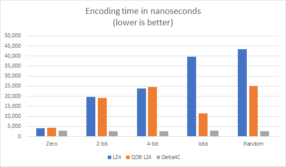
The two important metrics we are looking at are compression time:

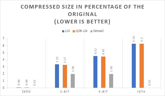
and compressed size:

The immediate, obvious, difference is that Delta4C encoding time is constant and always faster than LZ4 and QDB LZ4. The difference speed is up to 12X with QDB LZ4 and 24X with vanilla LZ4.

The second thing is that in these examples, Delta4C does much better than LZ4 even being able to recognize the obvious iota pattern to achieve “perfect compression”. The iota pattern is a perfect example of how you can beat dictionary compression for timeseries data.

When will Delta4C be available?

We’re currently in the final stages of testing of Delta4C. We are making sure our different strategies don’t generate obvious anti-patterns. We’re also increasing the capabilities of Delta4C to detect patterns to achieve “perfect compression”.

If you are running a fully managed QuasarDB solution, you can contact your solutions architect to have Delta4C deployed to your instance at no extra cost.

If you are running QuasarDB on premises, we are currently aiming at general availability of Delta4C this summer.

As always, check out our community edition or learn more about our managed timeseries solution.