
What Quasar optimizes for
What makes two software products perform differently?
Sometimes one uses a better algorithm or has a better implementation: that is a genuine engineering advantage. More often, however, the difference comes from the tradeoffs each system makes. A benchmark shows the result of those choices, but not whether they are right for your workload.
Nobody wants a slower database. But if a query already completes in 100 milliseconds, how much would you pay to reduce it to 10? For most workloads, probably nothing.
When we started Quasar, we were very focused on performance and assumed that faster always meant better. We learned that performance is usually a threshold: below it, a product is disqualified; above it, further gains may have little value. Enterprise deals make this particularly easy to misread. The engineer running the benchmark may love the results, while everyone else involved still sees no reason to change. Performance can disqualify a product, but by itself it rarely justifies a migration.
This does not make performance unimportant: it changes the question. Performance engineering is about deciding which costs matter and whether an optimization still helps outside the benchmark. Cutting a query from 5 milliseconds to 2.5 is not necessarily a win if it requires much more memory or interferes with other workloads. The query is faster, but the system may be worse.
Quasar comes from a particular set of requirements. We built it for very large, continuously changing datasets that may span several servers. Our users ingest data while querying it, with several workloads competing for the same resources. We therefore cannot optimize solely for the latency of one query running on an idle machine.
In the first part of this article, we explain several design choices that follow from these requirements. In the second, we compare Quasar with DuckDB and examine how those choices appear in benchmarks. We chose DuckDB because it is popular, exceptionally well implemented, and generally makes sensible design and algorithmic choices.
The choices we made
Quasar is not a local database
Quasar uses a client/server architecture because it is designed to scale beyond a single machine. Data can be distributed across multiple servers, and query work can be sent to the servers that hold the relevant data and executed in parallel.
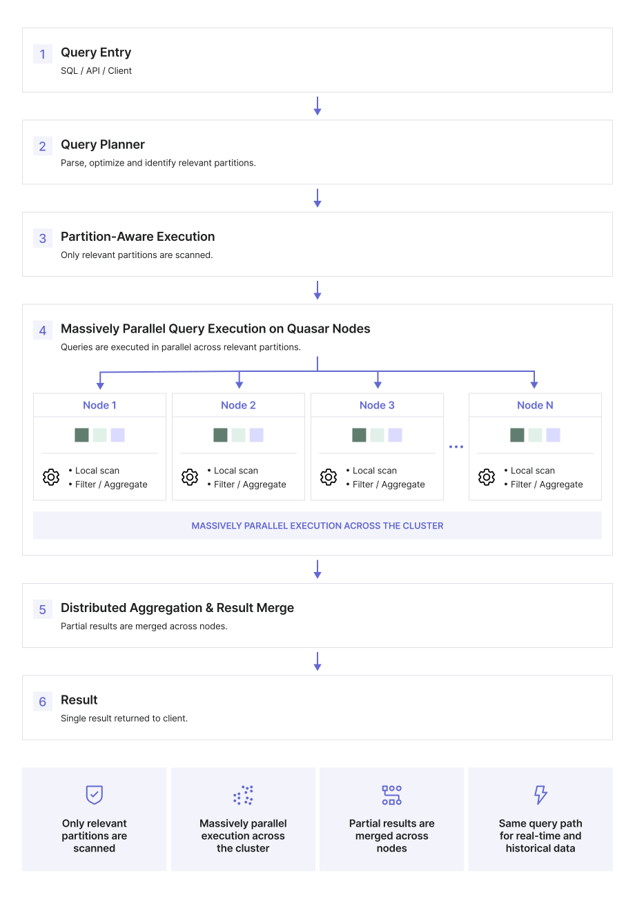
This architecture has a fixed cost. The client identifies where the data lives, divides the query into smaller tasks, and sends them across the network. This happens even when the client and server are in the same data center.
For a large query, that overhead is usually small compared with the work being performed. For a query that would otherwise complete in a fraction of a millisecond, it can dominate the result.
DuckDB, for example, makes a different tradeoff. It runs inside the application process and reads local data directly, without a network round trip or distributed query preparation. That gives it a genuine advantage over local datasets for small queries.
Quasar accepts this minimum latency because it is built to serve datasets and workloads that may span several machines. As the query grows, its initial cost remains relatively stable while more of the work can be distributed across the cluster.
We could bypass parts of the client path and report a lower number, but that would not represent how applications use Quasar.
In summary, DuckDB starts with local data; Quasar starts with the machinery needed to distribute data and computation across servers. Which architecture performs better depends on the size of the workload and where the data lives.
We schedule for concurrent workloads
A query engine divides work among multiple threads. Sometimes one thread finishes its assigned work while another still has a full queue. Work stealing allows the idle thread to take some of the remaining work. The query uses more of the available CPU and may finish sooner.
Work stealing works especially well when one query runs on an otherwise idle machine. Any unused core represents an opportunity to make that query faster.
Quasar scheduling is simple and predictable. An accurate assessment of the size of the data to be scanned for a given query is made, then the work is split into a configurable number of blocks, and data is processed to the server according to this block size. Let’s say you run an aggregation on a table, something like SELECT avg(x) FROM table. Let’s assume the table is split into 100 buckets, and you have a block size of 10. The client will send 10 units of work to the server. Those 10 units of work will be done in parallel as much as possible, depending on how many cores are assigned for queries on the server.
For the moment, Quasar does not use work stealing between workloads, doesn’t readjust as it processes the query, and doesn’t do any “work complexity” evaluation. Those things would improve performance at the cost of predictability and implementation complexity. You could argue that as a user, you don’t care about implementation complexity (“Why are we giving you guys money for?” is fair), but complexity does have a cost when it comes to central pieces of software such as query planning.
Now add continuous ingestion, several concurrent queries, and background work. Borrowing idle capacity improves the completion time of a single query, but it also makes the resources available to every workload less predictable. The fastest query may come at the expense of the others.
To summarize, we tend to favor predictability, fairness, and stability over unitary query performance. For the workloads we target, large datasets, concurrent queries, and continuous ingestion, we currently find that tradeoff more useful.
Indexing
Indexes can produce the most impressive improvements in a database benchmark. With the right index, a query that scans a large dataset may only need to read a small part of it. A ten-second query can become a 100-millisecond query.
The database pays for that speed elsewhere. An index occupies memory and disk. Every write may need to update it. Building, storing, and maintaining it becomes part of the cost of the whole dataset, even if only a few queries use it.
This matters more as the dataset grows: adding 10% to a small database may be trivial, but adding 10% to several petabytes is not. The index needs to create enough value across the workload to justify a permanent increase in storage and write cost.
Quasar uses small indexes which are mostly zone maps with extra information. A zone map records the minimum and maximum values found in a block of data, and helps with pruning.
A zone map will be not match for a specialized index for every query. If you frequently search for one value scattered throughout the dataset, a dedicated index may win by a wide margin. Zone maps offer a different balance: they remain compact, require little maintenance, and help many queries discard irrelevant data.
This does not mean that indexes are bad or that Quasar will never add more specialized ones. So far, for the size and shape of the datasets Quasar handles, we have favored broad improvements with low permanent costs over large improvements to occasional queries.
The relevant number is not only how much faster an index makes one query. It is also how much larger it makes the dataset, what it does to ingestion, and how often the workload benefits from it.
The cheapest cache operation can cost more later
A cache keeps frequently used data in memory so the database does not need to read it from storage again. When the cache fills, it needs to decide what to evict.
The classic least recently used (LRU) policy evicts the item that has been unused the longest. It is simple and inexpensive. It also has a weakness: a large scan can fill the cache with data read once, evicting smaller working sets that the system reads repeatedly.
After the scan finishes, the cache contains the end of that scan rather than the data the workload normally uses. The next queries must read their working sets from storage again. A policy that made each cache operation very cheap has caused much more expensive I/O.
Quasar uses LRU-2. Instead of considering only the most recent access, LRU-2 also tracks whether data has been accessed more than once. This makes LRU-2 scan resistant: it is less likely that a one-time scan will displace data with a history of repeated use.
LRU-2 requires more bookkeeping than LRU and can add a few microseconds to a small query. LRU-2 is also not always making a better decision than LRU. We could build a benchmark in which LRU wins: the result would be correct, but it would leave out the condition that motivated the choice.
Quasar accepts the small bookkeeping cost because storage I/O is much more expensive than a cache decision. For a system that scans large datasets while serving other queries, keeping the cache useful after the scan matters more than minimizing the cost of an ideal cache lookup.
Fast ingestion still has to produce usable data
Quasar uses a log-structured merge tree, or LSM, as the basis of its storage engine. Rather than updating data in place for every write, an LSM writes new data efficiently and reorganizes it later through compaction. This design supports the sustained write rates we expect from a high-ingest database.
The tradeoff is write amplification. Compaction reads and rewrites data, so the storage system may write several bytes for every byte received from the client. A different storage design might write less over the lifetime of the data, but handle a continuous stream of new records less efficiently.
For Quasar, this is a deliberate choice. Our users may ingest hundreds of billions of rows per day, and queries must continue while that data arrives. Sustained write throughput matters enough to accept additional work later.
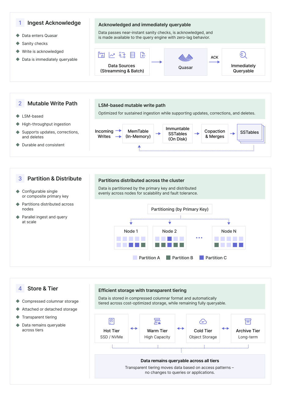 But raw write throughput does not tell the whole story. Quasar uses transactions, stores checksums, and checks data structures on both the write and read paths. These operations consume CPU and move additional bytes. Removing them could improve a benchmark that measures how quickly a system accepts input.
It could also leave corruption undetected or let a partial write appear complete. In that case, the system has not eliminated the cost. It has moved it to recovery, diagnosis, or a later query that can no longer trust the data it reads.
We count these checks as part of ingestion because writing data involves more than just placing bytes in storage. It means committing data that Quasar can find, verify, and read later. A comparison that disables those checks may still measure something useful, but it measures a weaker operation.
The trade-off here is not simply between write speed and correctness. The LSM itself is a performance choice: it favors high ingestion rates and accepts write amplification. Transactions, checksums, and structural checks define what Quasar promises once it reports that a write has succeeded.
Performance benchmarks!
Here comes the part everybody loves: numbers, a loser and a winner! Spoiler alert: there’s no winner.
We’re going to run a series of simple queries and explain the performance difference between DuckDB and QuasarDB. Both QuasarDB and DuckDB are written in C++ and are column-oriented. Duck is an engine we know: we built a DuckDB plugin that combines DuckDB’s flexibility with Quasar’s scale, including the ability to push parts of a query down to Quasar when Quasar can execute them more efficiently.
DuckDB runs in process and works particularly well with local data. Quasar uses a remote client-server path and prepares queries to distribute them across a cluster. Comparing the two makes the fixed cost of Quasar’s architecture visible, then shows how the balance changes as queries and datasets grow.
This is not an attempt to deliver a reproducible, scientific benchmark of which database is fastest, and it does not pretend to be exhaustive. The goal is to give you an idea of each system’s performance profile. You’ll see that we kept the queries and workload simple to make it easier to dissect differences.
Methodology
We run both systems on the same hardware and query the same source data. DuckDB runs locally in the benchmark process. Quasar uses its normal client/server path, including query preparation and remote calls, even when the server runs on the same network.
The tests are run on a workstation: Intel i9-10900KF, 64 GiB of RAM, consumer-grade SSD, and we are running Windows 11.
We compared DuckDB 1.5.4 vs QuasarDB 3.14.3. We run the same query 5 times and take the median, which means we’re comparing only hot queries. In both cases, schemas are configured to be optimal for each database, but neither has indexes (apart from built-in zone maps). Tables for Quasar are also only partitioned by time to avoid giving Quasar an unfair advantage, because DuckDB doesn’t support user-defined partitioning of native tables at the time of this writing.
We are simulating temperature capture on machines, each row is a timestamp, a machine ID, and temperature. Temperature is an arbitrary integer value that doesn’t try to be anything realistic, and is pseudo random with an attempt to be “realistic”. The data set is about 200 million rows, which is guaranteed to fit in the RAM of the test machine (to avoid putting the Duck too much at a disadvantage), but large enough so that naive aggregation algorithms won’t work.
Here is the Quasar query to create the table:
CREATE TABLE temperature_readings (
    $timestamp TIMESTAMP,
    machine_id INT64,
    temperature INT64)
SHARD_SIZE = 5000s;
Ingestion
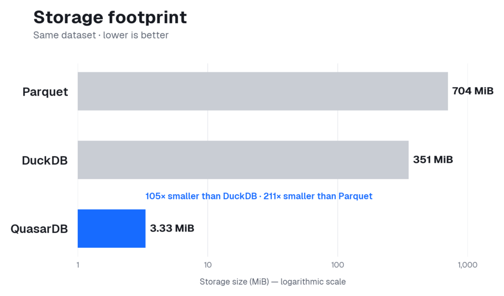
DuckDB can import our parquet file in 6.8s, and the disk usage for that is 351 MiB, which is fairly decent given that the parquet files combined are about 700 MiB.
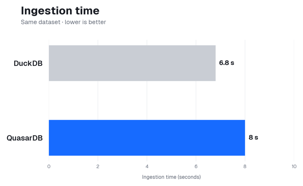
QuasarDB can import the file in 8s, and the disk usage for that is 3.33 MiB. We used synchronous writes (fully commited on function return), not asynchronous writes (delayed, optimized writes with immediate visibility). Regarding the compression ratio, it’s not a typo. Seems Delta4C, our compression, is detecting the patterns in the synthetic data and replacing them with adequate generators. That’s good! It seems we still have an edge around what is essentially one of our key selling point.
 Back to the benchmark. Does this mean that DuckDB ingest the data about 15% faster than QuasarDB? Yes in this benchmark, but in the general sense, no.
In this (relatively) small ingestion test, Quasar is paying a huge overhead: chunk the data, serialize it, and send it over the network, to have the server then deserialize it, recompress it, and store it in a LSM. Whereas DuckDB does a local import over a persisted database organized as a single file.
The tradeoff is that Quasar can be spread over several different servers in a cluster and the storage limit is how much storage you can buy. DuckDB is a local database that expects your file to be mappable into memory.
Simple queries
How fast can a “small data” query go?
SELECT
    MIN(temperature),
    MAX(temperature),
    AVG(temperature)
FROM temperature_readings
IN RANGE('2026-01-01 12:00:00', '2026-01-01 12:10:00')
WHERE machine_id = 42;
On DuckDB this takes 24ms, on QuasarDB 30ms. This gives us an idea of the fixed cost of each architecture. DuckDB performs well here because it runs in the benchmark process and begins executing without a network round-trip. Quasar must prepare the query and cross the client/server boundary before it can return a result.
The result tells us the minimum practical latency of each system in this configuration. It does not tell us how either system behaves when the query processes more data or when the workload no longer fits comfortably on one machine.
SELECT
    MIN(temperature),
    MAX(temperature),
    AVG(temperature)
FROM temperature_readings;
In this query, DuckDB needs 102ms, whereas QuasarDB takes 30ms. QuasarDB zone-maps are richer than DuckDB’s, and they fully kick in in that scenario. This is typically the kind of scenario where the marketing department would say “QuasarDB is 4 times faster than DuckDB” and be technically correct (the best kind of correct), but it’s not a query that is that useful. Does this mean you should always ignore performance claims from vendors?
Let’s look into queries that are still simple, but closer to what you’d ask a database on a day-to-day basis.
Queries with a bit more muscle
We’re not getting too crazy here; we’re just going to aggregate the 200M rows into a fairly low-cardinality group and see if we can observe a significant performance difference. The query is designed to force scanning all columns.
The cardinality is intentionally kept low to give each engine a chance to optimize rather than relying on pruning and raw I/O.
SELECT
    machine_id,
    MIN(temperature),
    MAX(temperature),
    AVG(temperature)
FROM temperature_readings
GROUP BY machine_id
ORDER BY machine_id;
Here are the results: DuckDB 217ms, QuasarDB 223ms. Which means DuckDB is 2.6% faster, while Quasar has to make a remote call, deserialize, and merge the responses. It’s fair to say the performance level is identical, which is not unsurprising because under the hood, both engines use a perfect hashing strategy for this specific case.
For the following query, also fairly low cardinality:
SELECT
    temperature, count(temperature)
    FROM temperature_readings
    GROUP BY temperature;
DuckDB 112ms, QuasarDB 80ms. Not a meaningful difference, but the marketing department won’t care. They will tell you we’re faster. And that’s all you need to know. We’re faster!
What should you take from this benchmark?
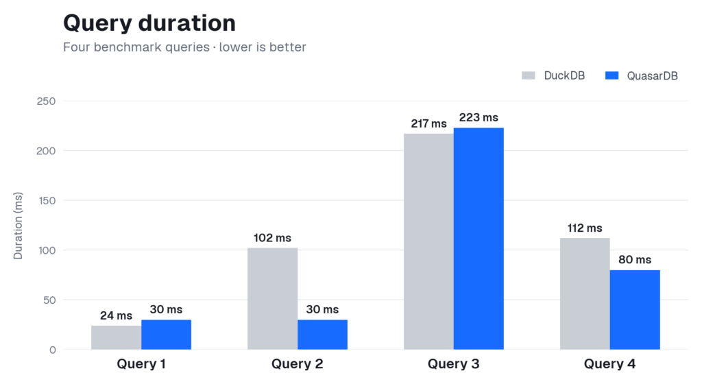 The purpose was never to declare a winner. It was to understand why two well-engineered (ahem) products perform differently and what their results reveal about their design. As it turns out, the differences are not dramatic on this workload: Quasar compresses much better, DuckDB ingests somewhat faster, and query performance is broadly comparable.
We kept the benchmark deliberately simple so that those differences would be easier to explain. That also limits what the results can tell you. A different query, data layout, level of concurrency, or access pattern could easily change the outcome.
The practical lesson is straightforward: test a workload that resembles the one you actually care about, and do not optimize before you know what matters. A few milliseconds on an isolated query should not decide a long-term architectural choice. Pick a system whose design fits both your current constraints and where you expect the workload to go.
There is also a small twist: you do not necessarily have to choose. Quasar’s has two query engines: the native one, highly optimized for numerical data workloads and timeseries operations, and a high-performance OLAP interface built on DuckDB.
If you’d like to learn more about Quasar, get in touch with one of our engineers!